

前言
在最近的科研生活中,我时常遇上很有意思的小问题,在此我开一个专栏专门记录下我已经解决的和未曾解决的小灵感。
问题说明
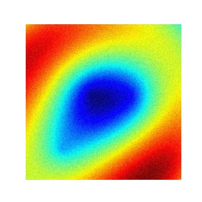
小灵感:在一块平面上,有$n$个振动源在产生振动,根据物理定律这些振动点会在平面上产生振动分布(激励分布),我将振幅数据采集,绘制出类似于图1中的分布图。此时,我想将振动分布图作为输入数据,振动点源的位置坐标作为输出数据,尤其需要注意的是,我不在模型中设置最后输出的点源的数量,也就是说模型最后输出的坐标的数量不是一成不变的。
我认为有意思的地方是——模型在一方面在做类似对点源数量的回归任务,输出预测的点源数量,一方面在分类的基础上进行回归任务,输出激励点源的位置坐标。
灵感假设
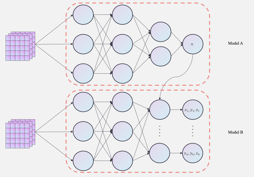
要在一个模型中做到这些是较为困难的,因此,我设想是否能组合两个模型构建为一个网络进行训练呢?假设$Model A$作为实现输出点源数量的部分,那么在$Model B$的输出层中,最后的输出层(线性层)的维度则由$Model A$(输出的点源数量)控制。这样就简单构建出了一个组合模型网络架构。
PS:经过后续的查阅资料,原来本文的这种组合模型网络架构已经有较多的相关工作了,常在多任务学习中运用,被称为级联神经网络。
如图2所示,能够更加清晰的看清楚模型的运作机制。
灵感小验证
下面是代码部分,我先采用了简单的线性层进行实验,测试我的小灵感是否能够实现。
import torch
import torch.nn as nn
import torch.nn.functional as F

class MLP4Number(nn.Module):
    def __init__(self, channel=3, hidden_dim=64, output_dim=1):
        super().__init__()
        self.fc1 = nn.Linear(channel, hidden_dim)
        self.fc2 = nn.Linear(hidden_dim, output_dim)

    def forward(self, x):
        x = F.relu(self.fc1(x))
        x = self.fc2(x)
        x = torch.round(x).clamp(min=1)
        return x

class MLP4Coordinate(nn.Module):
    def __init__(self, channel=10, hidden_dim=64, output_dim=1):
        super().__init__()
        self.fc1 = nn.Linear(channel, hidden_dim)
        self.fc2 = nn.Linear(hidden_dim, output_dim)
        self.number = output_dim

    def forward(self, x):
        x = F.relu(self.fc1(x))
        x = self.fc2(x)
        x = x.view(self.number, 3)
        return x

class MLP4TwoTask(nn.Module):
    def __init__(self, input_channels=256, hidden_dim=64, output_dim=1):
        super().__init__()
        self.input = input_channels ** 2
        self.hidden = hidden_dim
        self.number = MLP4Number(self.input, hidden_dim, output_dim)

    def forward(self, x):
        c = torch.tensor([])
        x = x.view(x.size(0), -1)
        n = self.number(x)
        for i in n:
            self.coordinate = MLP4Coordinate(self.input, self.hidden, output_dim=int(i))
            a = self.coordinate(x)
            c = torch.cat((c, a), dim=0)
        return n, c

if __name__ == '__main__':
    model = MLP4TwoTask()
    imgs = torch.randn(3, 256, 256)
    output = model(imgs)
    print(output)
下面是经过ChatGPT润色后的代码实现。
import torch
import torch.nn as nn
import torch.nn.functional as F

class MLP4Number(nn.Module):
    def __init__(self, in_dim: int, hidden_dim: int = 64, output_dim: int = 1):
        super().__init__()
        self.fc1 = nn.Linear(in_dim, hidden_dim)
        self.fc2 = nn.Linear(hidden_dim, output_dim)

    def forward(self, x: torch.Tensor) -> torch.Tensor:
        """
        输入:
            x: Tensor,shape = (batch_size, in_dim)
        输出:
            Tensor,shape = (batch_size, 1),经过 round 并 clamp(min=1)
        """
        x = F.relu(self.fc1(x))
        x = self.fc2(x)
        x = torch.round(x).clamp(min=1)
        return x.squeeze(-1)  # 返回 shape = (batch_size,)


class MLP4Coordinate(nn.Module):
    def __init__(self, in_dim: int, hidden_dim: int = 64, output_dim: int = 1):
        super().__init__()
        self.fc1 = nn.Linear(in_dim, hidden_dim)
        self.fc2 = nn.Linear(hidden_dim, output_dim * 3)
        # output_dim 表示“要预测几个三维点”,最终输出会 reshape 成 (output_dim, 3)

    def forward(self, x: torch.Tensor, num_points: int) -> torch.Tensor:
        """
        输入:
            x: Tensor,shape = (1, in_dim) 或 (batch=1, in_dim)  —— 单个样本
            num_points: int,表示要预测多少个 (x,y,z) 坐标点
        输出:
            Tensor,shape = (num_points, 3)
        """
        x = F.relu(self.fc1(x))
        x = self.fc2(x)  # shape = (1, num_points*3)
        x = x.view(num_points, 3)  # reshape 成 (num_points, 3)
        return x


class MLP4TwoTask(nn.Module):
    def __init__(self, input_size: int = 256, hidden_dim: int = 64):
        """
        input_size: 图像边长(如 256),网络的输入是 (batch, input_size, input_size)
        hidden_dim: MLP 隐藏层维度
        """
        super().__init__()
        self.input_dim = input_size * input_size  # 256*256
        self.hidden_dim = hidden_dim

        # 阶段一:预测要输出多少个点
        self.number_net = MLP4Number(in_dim=self.input_dim,
                                    hidden_dim=hidden_dim,
                                    output_dim=1)  # 单个数值

        # 注意:这里并不预先创建 MLP4Coordinate,因为 output_dim(坐标点数)是动态的。
        # 我们会在 forward 里按需实例化一个局部的 MLP4Coordinate

    def forward(self, x: torch.Tensor) -> (torch.Tensor, torch.Tensor):
        """
        输入:
            x: Tensor,shape = (batch_size, input_size, input_size)
        输出:
            num_list: Tensor,shape = (batch_size,) —— 每个样本预测的点的数量 (>=1)
            coords_all: Tensor,shape = (sum(num_list), 3) —— 把所有样本的坐标拼在一起
        """
        batch_size = x.size(0)
        device = x.device

        # 先把 (batch, H, W) -> (batch, H*W)
        x_flat = x.view(batch_size, -1)  # shape = (batch_size, input_dim)

        # 阶段一:预测每个样本要多少个点 (>=1)
        num_list = self.number_net(x_flat)  # shape = (batch_size,)
        # num_list 内的值是浮点取整后保证 ≥1,比如 [3., 1., 5., ...]

        coords_list = []
        for idx in range(batch_size):
            num_i = int(num_list[idx].item())  # 取出第 idx 个样本需要的点数 (Python int)

            # 注意:这里用临时变量,不要写成 self.coord_net,否则会被注册到 Module 里
            coord_net = MLP4Coordinate(in_dim=self.input_dim,
                                       hidden_dim=self.hidden_dim,
                                       output_dim=num_i).to(device)

            # 取出第 idx 个样本的扁平化向量,形状要是 (1, input_dim),方便 MLP4Coordinate 接受
            single_x = x_flat[idx].unsqueeze(0)  # shape = (1, input_dim)

            # 得到坐标:shape = (num_i, 3)
            coords_i = coord_net(single_x, num_points=num_i)
            coords_list.append(coords_i)

        # 把所有样本预测出来的坐标一起 cat,最终形状 = (sum(num_list), 3)
        coords_all = torch.cat(coords_list, dim=0)

        return num_list, coords_all


if __name__ == "__main__":
    # 示例运行
    model = MLP4TwoTask(input_size=256, hidden_dim=64)  # 如果有 GPU,就 .cuda()
    imgs = torch.randn(3, 256, 256)
    num_out, coords_out = model(imgs)
    print("Num per sample:", num_out)            # e.g. tensor([2., 5., 1.], device='cuda:0')
    print("All coords shape:", coords_out.shape) # (2+5+1, 3) = (8,3) 这种形式
验证实验
接下来我们将级联MLP改变为级联CNN,下面开始实验。
构建数据集
在本文中的所有数据都是采用了数值模拟的办法,下面是我们简要构建数据集的代码。
import numpy as np
import matplotlib.pyplot as plt
import os
import random
from matplotlib import cm  # 导入颜色映射模块

# 创建输出目录
output_dir = "data"
if not os.path.exists(output_dir):
    os.makedirs(output_dir)

# 波的参数
k = 0.2  # 波的频率
speed = 0.2  # 波的传播速度
nums = 100  # 生成数据数量
resolution = 400  # 图像分辨率

# 网格点
x = np.linspace(-10, 10, resolution)
y = np.linspace(-10, 10, resolution)
X, Y = np.meshgrid(x, y)

# 随机生成激励点位置
def generate_random_sources(num_sources):
    sources = []
    for _ in range(num_sources):
        x_pos = random.uniform(0, 1)  # 随机 x 坐标
        y_pos = random.uniform(0, 1)  # 随机 y 坐标
        sources.append(np.array([x_pos, y_pos]))
    return sources

# 生成波的幅度
def generate_wave(sources, frame):
    Z = np.zeros_like(X)  # 初始化波的幅度
    for center in sources:
        R = np.sqrt((X - center[0]) ** 2 + (Y - center[1]) ** 2)
        Z += np.sin(k * R - speed * frame)  # 叠加每个激励点的波
    return Z

# 生成并保存数据(添加高斯噪声)
def generate_and_save_data(num_sources, output_dir="route_data"):
    # 创建子目录
    npy_dir = os.path.join(output_dir, "npy")
    pic_dir = os.path.join(output_dir, "pic")
    os.makedirs(npy_dir, exist_ok=True)
    os.makedirs(pic_dir, exist_ok=True)

    for frame in range(nums):
        # 随机生成激励点位置
        sources = generate_random_sources(num_sources)

        # 生成波的幅度
        Z = generate_wave(sources, frame)

        # 将波形数据映射为 RGB 图像数据
        norm_z = (Z - Z.min()) / (Z.max() - Z.min())
        rgba_data = cm.jet(norm_z)
        rgb_data = rgba_data[..., :3]

        # 添加高斯噪声
        noise_std = 0.1  # 噪声强度,根据需要调整
        noise = np.random.normal(0, noise_std, rgb_data.shape)
        noisy_rgb = np.clip(rgb_data + noise, 0, 1)  # 限制在有效范围

        # 保存带噪声的npy文件
        npy_filename = os.path.join(npy_dir, f"{num_sources}_frame_{frame:03d}.npy")
        np.save(npy_filename, noisy_rgb)

        # 可视化并保存图片
        img_filename = os.path.join(pic_dir, f"{num_sources}_frame_{frame:03d}.png")
        plt.imshow(noisy_rgb)
        # 标记激励点
        for source in sources:
            x_idx = np.argmin(np.abs(x - source[0]))
            y_idx = np.argmin(np.abs(y - source[1]))
            plt.scatter(x[x_idx], y[y_idx], color='white', s=100, marker='x', alpha=0.6)  # 调整透明度
        plt.axis('off')
        plt.savefig(img_filename, bbox_inches='tight', pad_inches=0)
        plt.clf()

    print(f"Generated route_data for {num_sources} sources with Gaussian noise.")
    print(f"Saved route_data to {output_dir}")

# 生成带噪声的数据
generate_and_save_data(1)
generate_and_save_data(2)
generate_and_save_data(3)
在上述的代码中,我们设置波的频率为$k=0.2$,传播速度为0.2,每组数量为100,高斯噪声为0.1,每组的图像分辨率为$400 \times 400$,随机点的x和y的坐标范围均在$[0,1]$。其中,由于神经网络的本质其实就是一种函数映射$f(\cdot)$,所以我们可以随意构建具体坐标(因为只是要验证idea的可行性,无需太过严谨),通过构建在x和y的坐标范围内的坐标数据并将其作为文件名对Data进行重命名,得到最后的数据集。
PS(微操):无论坐标数据的范围,其实都可以将其归一化后输入网络中进行学习,前提是需要提取纪录下数据中的最大值与最小值用来还原回原坐标。
我们在训练过程中构建出Data内容为(Images,Coords)的数据集,其中Images为(batch,3,H,W),Coords为(batch,coords),Images Size为$400 \times 400$。
下面是构建数据集部分的代码:
class NpyDataset(Dataset):
    def __init__(self, data_dir: str):
        super().__init__()
        self.file_paths = glob.glob(os.path.join(data_dir, "*.npy"))
        self.file_paths.sort()

    def __len__(self):
        return len(self.file_paths)

    def __getitem__(self, idx: int):
        file_path = self.file_paths[idx]
        filename = os.path.basename(file_path)

        # 加载 .npy 文件内容
        np_array = np.load(file_path)  # e.g. shape = (400, 400, 3)

        # 如果是三通道(H, W, 3),转成 (3, H, W)
        if np_array.ndim == 3:
            # 假设最后一维是 channel
            data_tensor = torch.from_numpy(np_array).permute(2, 0, 1).float()
        elif np_array.ndim == 2:
            # 如果是单通道(H, W),加一个通道维 (1, H, W)
            data_tensor = torch.from_numpy(np_array).unsqueeze(0).float()
        else:
            # 如果数据有其他维度,就根据实际情况处理
            raise ValueError(f"Unsupported npy shape: {np_array.shape}")

        # 从文件名解析坐标(不变)
        name_without_ext = os.path.splitext(filename)[0]
        parts = name_without_ext.split("_")
        coords = []
        for i in range(0, len(parts), 2):
            x = float(parts[i]);
            y = float(parts[i + 1])
            coords.append([x, y])
        coord_tensor = torch.tensor(coords, dtype=torch.float32)

        return data_tensor, coord_tensor

def variable_collate_fn(batch):
    """
    自定义 collate_fn,用于处理每个样本 label (coord) 长度不同的情况。
    batch 是 list of (data_tensor, coord_tensor)。

    返回:
      data_batch: Tensor, 将 data_tensor 堆叠,形状 = (batch_size, ...)
      coords_list: List of Tensors, 每个 coord_tensor 形状 = (Ni, 2)
    """
    data_list, coords_list = zip(*batch)
    data_batch = torch.stack(data_list, dim=0)
    return data_batch, list(coords_list)
构建级联CNN
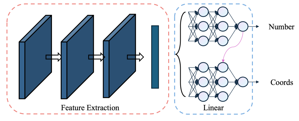
如图3所示,我们先采用卷积操作提取图片的特征信息,然后将特征信息输入线性层进行进一步的学习和变化,最后输出我们想要得到的数据。其中,在Feature Extraction中,为了使得网络层数能够更多,我们采用了由残差连接构成的残差块,经过堆叠构成总体的卷积提取部分。
PS:由于图3中模型的表达能力有限,下方的代码仅仅只表示模型搭建的基本思路,在复现过程中请根据自己的需求对模型进行模块的添加,本文中的所有代码均放置于Github中,有需要浮现者可以前往我的Github上查看完整的代码。(https://github.com/MAOJIUTT/Cascade-Neural-Networks)
下面是模型的代码
class ResBlock(nn.Module):
    def __init__(self, channels: int):
        super().__init__()
        self.conv1 = nn.Conv2d(channels, channels, kernel_size=3, padding=1, bias=False)
        self.bn1 = nn.BatchNorm2d(channels)
        self.conv2 = nn.Conv2d(channels, channels, kernel_size=3, padding=1, bias=False)
        self.bn2 = nn.BatchNorm2d(channels)

    def forward(self, x: torch.Tensor) -> torch.Tensor:
        identity = x
        out = self.conv1(x)
        out = self.bn1(out)
        out = F.relu(out, inplace=True)
        out = self.conv2(out)
        out = self.bn2(out)
        out += identity
        out = F.relu(out, inplace=True)
        return out


class CNN4TwoStage(nn.Module):
    def __init__(
        self,
        in_channels: int = 1,
        base_channels: int = 32,
        num_resblocks: int = 2,
        max_points: int = 10,
        hidden_dim: int = 128
    ):
        super().__init__()
        self.in_channels = in_channels
        self.base_channels = base_channels
        self.max_points = max_points
        self.hidden_dim = hidden_dim

        # backbone
        self.conv_start = nn.Sequential(
            nn.Conv2d(in_channels, base_channels, kernel_size=3, padding=1, bias=False),
            nn.BatchNorm2d(base_channels),
            nn.ReLU(inplace=True)
        )
        res_blocks = []
        for _ in range(num_resblocks):
            res_blocks.append(ResBlock(base_channels))
        self.residual_layers = nn.Sequential(*res_blocks)
        self.global_pool = nn.AdaptiveAvgPool2d((1,1))
        self.fc_feature = nn.Linear(base_channels, hidden_dim)

        # Number Head
        self.number_fc = nn.Linear(hidden_dim, 1)

        # Coordinate Head (改为 max_points * 2)
        self.coord_fc = nn.Linear(hidden_dim, max_points * 2)

    def forward(self, x: torch.Tensor) -> (torch.Tensor, torch.Tensor):
        """
        输入:
            x: (batch, in_channels, H, W)
        输出:
            num_list: (batch,) 整数型,预测的每张图要输出几个点
            coords_all: (sum_i Ni, 2) 所有样本拼接后的 (x,y) 坐标
        """
        batch_size = x.size(0)
        device = x.device

        # backbone 提取特征
        out = self.conv_start(x)           # (batch, base, H, W)
        out = self.residual_layers(out)    # (batch, base, H, W)
        out = self.global_pool(out)        # (batch, base, 1, 1)
        out = out.view(batch_size, -1)     # (batch, base)
        feat = F.relu(self.fc_feature(out))# (batch, hidden_dim)

        # Number Head
        num_pred = self.number_fc(feat)    # (batch,1)
        num_pred = torch.round(num_pred).clamp(min=1)  # 保证 ≥1
        num_list = num_pred.squeeze(-1).long()         # (batch,)

        # Coordinate Head → (batch, max_points*2)
        coord_pred = self.coord_fc(feat)   # (batch, max_points*2)

        coords_list = []
        for i in range(batch_size):
            n_i = int(num_list[i].item())
            if n_i > self.max_points:
                n_i = self.max_points
            # 取前 n_i*2 个数,reshape 为 (n_i,2)
            coords_i = coord_pred[i, : n_i * 2].view(n_i, 2)
            coords_list.append(coords_i)

        # 把所有样本的 coords_i 在第 0 维拼起来 -> (sum_i n_i, 2)
        coords_all = torch.cat(coords_list, dim=0)
        return num_list, coords_all
阶段性训练(冻结-微调策略)
由于级联CNN是多任务结构,是一个典型的多任务学习模型(Multi-Task Learning,MTL),拥有两个部分——主干网络(Backbone)和任务分支(Head)。主干网络用于提取共享特征,任务分支则是完成对应需要完成的任务。其中,在本文的多任务结构中有两个关联的学习阶段,阶段1 为 Number Head 预测的是每张图中目标的个数;阶段2 为 Coordinate Head 预测的是目标的坐标,而它依赖于阶段1 Number Head的预测结果。因此,可以认为如果 Number Head 预测不准,那么 Coordinate Head 的训练会受影响(如点数不对导致配对错误)。所以,我们可以采用如下两段式训练策略。
第一阶段:冻结 Coordinate Head ,只优化数量预测,代码如下。
def train_number_head(model, loader, optimizer, epochs=10):
    model.train()

    # 冻结坐标预测头
    for param in model.coord_fc.parameters():
        param.requires_grad = False

    mse_num = nn.MSELoss()

    for epoch in range(epochs):
        epoch_loss = 0.0
        for x_batch, coords_list in loader:
            x_batch = x_batch.to(device)
            num_target = torch.tensor(
                [coords.shape[0] for coords in coords_list],
                dtype=torch.float32, device=device
            )

            num_pred, _ = model(x_batch)

            loss = mse_num(num_pred.float(), num_target)

            optimizer.zero_grad()
            loss.backward()
            optimizer.step()

            epoch_loss += loss.item()

        print(f"[Number Head] Epoch [{epoch+1}/{epochs}]  Loss: {epoch_loss:.6f}")
第二阶段:解冻 Coordinate Head ,可选冻 Number Head ,代码如下。
def train_coord_head(model, loader, optimizer, epochs=10, lambda_coord=1.0, freeze_number_head=False):
    model.train()

    # 解冻坐标头
    for param in model.coord_fc.parameters():
        param.requires_grad = True

    # 可选:冻结数量预测头
    if freeze_number_head:
        for param in model.number_fc.parameters():
            param.requires_grad = False

    mse_num = nn.MSELoss()
    mse_coord = nn.MSELoss()

    for epoch in range(epochs):
        total_loss_num, total_loss_coord = 0.0, 0.0

        for x_batch, coords_list in loader:
            x_batch = x_batch.to(device)

            num_target = torch.tensor(
                [coords.shape[0] for coords in coords_list],
                dtype=torch.float32, device=device
            )

            coords_target_all = torch.cat(
                [coords.to(device) for coords in coords_list], dim=0
            )

            num_pred, coords_pred_all = model(x_batch)

            loss_num = mse_num(num_pred.float(), num_target)
            loss_coord = mse_coord(coords_pred_all, coords_target_all)

            total_loss = loss_num + lambda_coord * loss_coord

            optimizer.zero_grad()
            total_loss.backward()
            optimizer.step()

            total_loss_num += loss_num.item()
            total_loss_coord += loss_coord.item()

        print(f"[Coord Head] Epoch [{epoch+1}/{epochs}]  NumLoss: {total_loss_num:.6f}  CoordLoss: {total_loss_coord:.6f}")
但是在训练过程中计算Loss值时,仍然会遇上点数不对导致配对错误的问题,本篇Blog目前未能解决该问题,所以在本文中我所采用的解决方法是分段式训练模型,先将模型中预测激励点数量的模块部分训练到90%以上的准确率,然后再在这个基础上训练预测坐标部分的模型,这样就能够保证一定的模型预测准确率。
PS:本Blog中未解决的问题部分我会在暑期中尝试解决。
损失函数
在训练过程中,损失函数是尤为重要的,但是在这个网络架构中,模型的输出维度是动态的,在维度上无法很好的与数据的标签维度对应,因此无法直接对其进行求损失。结合本文的训练思路,我采用逐数量一一对应求Loss损失值。
具体意思就是,当模型输出维度与数据标签的维度不匹配时,我只需要根据较小那一部分的输出维度作为计算Loss损失值时的维度。因为模型的输出维度与数据标签维度不同时会存在两种情况,一是模型的输出维度小于数据标签维度(预测点的数量小于目标数量),二是模型的输出维度大于数据标签维度(预测点的数量大于目标数量)。所以为了保持维度上的统一以方便计算Loss损失值,我决定根据较小那一部分的输出维度作为计算Loss损失值时的维度。
所以我们将第二阶段的代码修改如下:
def train_coord_head(model, loader, optimizer, epochs=10, lambda_coord=1.0, freeze_number_head=False, coord_eps=0.5):
    model.train()

    for param in model.coord_fc.parameters():
        param.requires_grad = True

    if freeze_number_head:
        for param in model.number_fc.parameters():
            param.requires_grad = False

    mse_num = nn.MSELoss()
    mse_coord = nn.MSELoss()

    for epoch in range(epochs):
        total_loss_num, total_loss_coord = 0.0, 0.0
        correct_count_num = 0
        total_count_num = 0

        correct_count_coord = 0
        total_count_coord = 0

        for x_batch, coords_list in loader:
            x_batch = x_batch.to(device)

            num_target = torch.tensor(
                [coords.shape[0] for coords in coords_list],
                dtype=torch.float32, device=device
            )

            coords_target_all = torch.cat(
                [coords.to(device) for coords in coords_list], dim=0
            )

            num_pred, coords_pred_all = model(x_batch)

            # ===== 点数预测 =====
            loss_num = mse_num(num_pred.float(), num_target)

            pred_rounded = torch.round(num_pred).clamp(min=1, max=model.max_points)
            correct_count_num += (pred_rounded == num_target).sum().item()
            total_count_num += len(num_target)

            # ===== 坐标预测 =====
            pred_coords_split = []
            target_coords_split = []
            idx_pred = 0
            idx_target = 0
            for i in range(len(coords_list)):
                coords_target_i = coords_list[i].to(device)
                n_target = coords_target_i.shape[0]
                n_pred = int(pred_rounded[i].item())

                coords_pred_i = coords_pred_all[idx_pred: idx_pred + n_pred]
                idx_pred += n_pred
                idx_target += n_target

                # 取最小长度
                n_common = min(n_pred, n_target)
                if n_common > 0:
                    coords_pred_i = coords_pred_i[:n_common]
                    coords_target_i = coords_target_i[:n_common]

                    pred_coords_split.append(coords_pred_i)
                    target_coords_split.append(coords_target_i)

                    # ==== 准确率统计 ====
                    dist = torch.norm(coords_pred_i - coords_target_i, dim=1)
                    correct_count_coord += (dist < coord_eps).sum().item()
                    total_count_coord += n_common

            if pred_coords_split:
                coords_pred_used = torch.cat(pred_coords_split, dim=0)
                coords_target_used = torch.cat(target_coords_split, dim=0)
                loss_coord = mse_coord(coords_pred_used, coords_target_used)
            else:
                loss_coord = torch.tensor(0.0, device=device)

            total_loss = loss_num + lambda_coord * loss_coord

            optimizer.zero_grad()
            total_loss.backward()
            optimizer.step()

            total_loss_num += loss_num.item()
            total_loss_coord += loss_coord.item()

        acc_num = correct_count_num / total_count_num if total_count_num > 0 else 0.0
        acc_coord = correct_count_coord / total_count_coord if total_count_coord > 0 else 0.0

        print(f"[Coord Head] Epoch [{epoch+1}/{epochs}]  NumLoss: {total_loss_num:.6f}  CoordLoss: {total_loss_coord:.6f}  "
              f"NumAcc: {acc_num:.4f}  CoordAcc(@{coord_eps}): {acc_coord:.4f}")
可以看到,在改进后的代码中,我们在判断坐标预测的准确率的时候,设置了coord_eps参数为0.5,作为距离容差(距离容忍度的差值),用其作为距离容差计算得到的Coord Acc值则表示为预测点距离真实点的欧几里得距离小于0.5的预测点的比例。
模型的性能
由于在模型的训练过程中,采用图3的网络架构训练的效果不是很好,我们重新根据图3的基本思路在特征提取阶段添加了下采样的过程,以及在坐标预测分支中将线性层替换为残差MLP结构,具体代码如下:
class ResBlock(nn.Module):
    def __init__(self, channels: int):
        super().__init__()
        self.conv1 = nn.Conv2d(channels, channels, kernel_size=3, padding=1, bias=False)
        self.bn1 = nn.BatchNorm2d(channels)
        self.conv2 = nn.Conv2d(channels, channels, kernel_size=3, padding=1, bias=False)
        self.bn2 = nn.BatchNorm2d(channels)

    def forward(self, x):
        identity = x
        out = F.relu(self.bn1(self.conv1(x)), inplace=True)
        out = self.bn2(self.conv2(out))
        return F.relu(out + identity, inplace=True)

class DownBlock(nn.Module):
    def __init__(self, in_channels, out_channels, dropout_rate=0.0, use_resblock=True):
        super().__init__()
        self.down = nn.Sequential(
            nn.Conv2d(in_channels, out_channels, kernel_size=4, stride=2, padding=1, bias=False),
            nn.BatchNorm2d(out_channels),
            nn.ReLU(inplace=True),
        )
        self.res = ResBlock(out_channels) if use_resblock else nn.Identity()
        self.dropout = nn.Dropout2d(dropout_rate) if dropout_rate > 0 else nn.Identity()

    def forward(self, x):
        x = self.down(x)
        x = self.res(x)
        x = self.dropout(x)
        return x

class ResidualCoordHead(nn.Module):
    def __init__(self, hidden_dim, max_points):
        super().__init__()
        self.max_points = max_points

        self.fc1 = nn.Linear(hidden_dim, hidden_dim)
        self.norm1 = nn.LayerNorm(hidden_dim)
        self.dropout1 = nn.Dropout(0.2)

        self.fc2 = nn.Linear(hidden_dim, hidden_dim // 2)
        self.norm2 = nn.LayerNorm(hidden_dim // 2)
        self.dropout2 = nn.Dropout(0.2)

        self.output_layer = nn.Linear(hidden_dim // 2, max_points * 2)
        self.shortcut = nn.Linear(hidden_dim, hidden_dim // 2)

    def forward(self, x):
        residual = self.shortcut(x)
        x = F.relu(self.norm1(self.fc1(x)))
        x = self.dropout1(x)
        x = F.relu(self.norm2(self.fc2(x)))
        x = self.dropout2(x)
        return self.output_layer(x + residual)

class CNN4TwoStage(nn.Module):
    def __init__(
        self,
        in_channels=1,
        base_channels=32,
        max_points=10,
        hidden_dim=128,
        num_down_blocks=6,
        dropout_rate=0.3,
        use_resblock=True,
    ):
        super().__init__()
        self.max_points = max_points

        # 构建 DownBlock 列表
        self.down_blocks = nn.ModuleList()
        channels = [in_channels] + [base_channels * (2 ** i) for i in range(num_down_blocks)]
        for i in range(num_down_blocks):
            self.down_blocks.append(DownBlock(
                in_channels=channels[i],
                out_channels=channels[i + 1],
                dropout_rate=dropout_rate,
                use_resblock=use_resblock
            ))

        self.global_pool = nn.AdaptiveAvgPool2d((1, 1))
        final_channel = channels[-1]

        self.fc_feature = nn.Sequential(
            nn.Flatten(),
            nn.Linear(final_channel, hidden_dim),
            nn.ReLU(inplace=True),
            nn.Dropout(dropout_rate),
        )

        self.number_fc = nn.Linear(hidden_dim, 1)
        self.coord_fc = ResidualCoordHead(hidden_dim, max_points)

    def forward(self, x):
        batch_size = x.size(0)
        device = x.device

        for block in self.down_blocks:
            x = block(x)

        x = self.global_pool(x)
        feat = self.fc_feature(x)

        num_pred = self.number_fc(feat).squeeze(-1)  # (B,)
        coord_pred = self.coord_fc(feat)  # (B, max_points * 2)

        coords_list = []
        for i in range(batch_size):
            n_i = int(torch.round(num_pred[i]).clamp(1, self.max_points).item())
            coords_i = coord_pred[i, :n_i * 2].view(n_i, 2)
            coords_list.append(coords_i)

        coords_all = torch.cat(coords_list, dim=0) if coords_list else torch.empty(0, 2, device=device)
        return num_pred, coords_all
我大概做了一些简单的对比实验来测量模型的基本性能,再进行训练前,为了实验的可复现性,我设置了随机种子进行初始化模型参数,代码如下,记住这个函数需要放在导库后以及所有函数前,并且需要在所有函数前调用。
def set_seed(seed: int = 42):
    random.seed(seed)
    np.random.seed(seed)
    torch.manual_seed(seed)
    torch.cuda.manual_seed(seed)
    torch.cuda.manual_seed_all(seed)  # if using multi-GPU
    torch.backends.cudnn.deterministic = True
    torch.backends.cudnn.benchmark = False

set_seed()
特别注意本文中只探究Idea的可实现性,而不做严谨的探讨(比如说还需要在验证集上进行测试等)
效果验证
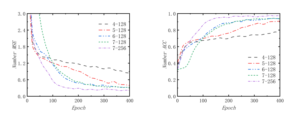
如图4,我们能够看到阶段1中的MSE损失曲线和预测准确率曲线,均能看到loss都在下降,我们先进行横向对比,也就是固定隐藏层为128,然后对比在不同Block数量下的收敛情况;再固定Block数量为7,然后再对比不同隐藏层数量下的收敛情况。根据MSE损失图像,得到结论——在相同隐藏层下增加Block的数量会加快收敛速度和收敛效果;在相同Block数量下增加隐藏层维度同样也会加快收敛速度和收敛效果。 当然,也可以看到准确率的曲线也符合MSE损失图像得到的结论。
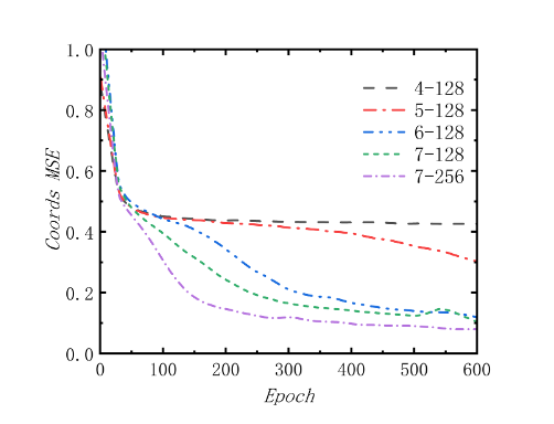
如图5,由阶段2中的MSE损失图像依旧可以得到阶段1中的结论,同样证明了“在相同隐藏层下增加Block的数量会加快收敛速度和收敛效果;在相同Block数量下增加隐藏层维度同样也会加快收敛速度和收敛效果”。
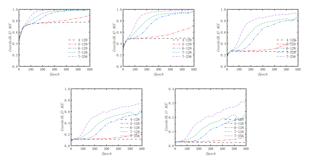
如图6,我还探究了在设置的不同距离容差下,阶段2的准确率情况。我发现模型预测的精度大概是在0.1~0.2左右,因为模型在距离容差为0.5,0.4,0.3的情况下都能够保持90%以上高准确率的效果,在距离容差为0.2时,模型的准确率下降明显,尽管同样有接近80%的准确率,但是当容差为0.1时,模型的准确率断崖式下降,虽然使用7-256(Block数量为7,隐藏层维度为256)的模型的准确率比其他模型准确率要高得多,但是准确率仍然很低(低于35%)。所以能够知道模型的坐标预测精度为0.1~0.2左右,总体上预测效果不错。
性能指标
接下来我会以数值的形式来研究模型的效果,但是具体数值表示的意义就不再赘述。
| Blocks | Hidden Dim | Num MSE | Coord MSE | Num Acc | Num Time | Coord Time | Param |
| 4 | 128 | 0.714229 | 0.418045 | 84.00% | 499 | 807 | 2.2M |
| 5 | 128 | 0.316047 | 0.296123 | 94.67% | 513 | 814 | 8.8M |
| 6 | 128 | 0.243847 | 0.113514 | 97.67% | 537 | 822 | 34.8M |
| 7 | 128 | 0.250646 | 0.103853 | 97.00% | 542 | 889 | 138.9M |
| 7 | 256 | 0.159434 | 0.070690 | 99.33% | 579 | 904 | 139.3M |
模型7-256在各方面均远优于模型4-128,其中Num MSE下降了约78.87%,Coord MSE下降了约83.25%,Num Acc提高了约15.33%,但是时间开销成本分别只增加了16%和12%。
| Blocks | Hidden Dim | Coord(0.5) | Coord(0.4) | Coord(0.3) | Coord(0.2) | Coord(0.1) |
| 4 | 128 | 81.65% | 53.01% | 29.52% | 14.09% | 4.24% |
| 5 | 128 | 90.39% | 73.82% | 49.58% | 25.25% | 7.59% |
| 6 | 128 | 99.83% | 96.95% | 86.80% | 62.75% | 23.74% |
| 7 | 128 | 100% | 97.97% | 88.18% | 66.78% | 25.50% |
| 7 | 256 | 100% | 99.66% | 95.81% | 77.76% | 36.29% |
如上表示,在确定精度的时,模型7-256依旧要在各方面远优于模型4-128,当距离容差分别为0.5,0.4,0.3,0.2,0.1时,预测的准确率(精准度)分别提高了18%,46%,66%,63%,32%。
小结
总体上来看,本文的级联神经网络的Idea是可行的,但是在具体的实验过程中还是会有一些不严谨的地方存在,例如生成数据集的时候采用的随机坐标设置,这个也算上另外一种数据污染吧,还有在实验中没有设置验证集和测试集,当然还有很多其他的问题,在此就不再赘述,最后再次强调本文只是用于验证Idea的可实现性,并非是一篇严谨的论文或者技术分享帖,感谢理解。
Comments NOTHING